Aleo Roadmap 2025 and In-Depth Exploration of Varuna

TL;DR

Recently, Aleo released their roadmap for 2025. We analyze the possible algorithms Varuna will use to achieve this goal.

Varuna is the current proof system for snarkVM in Aleo, used to prove the correctness of program execution (written in the Leo language). It reduces the problem of proving the correctness of one or more program executions to proving an R1CS problem, with the underlying proof leveraging the sum-check protocol for univariate polynomials.

1. Roadmap 2025

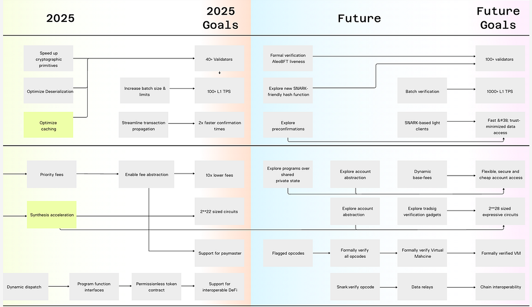
Aleo officially released the 2025 roadmap, as shown in the figure below. The goal for 2025 is to support circuits of size 2²², with plans to support circuits of size 2²⁸ in the future, which poses significant challenges for memory and computational power.
To achieve this goal, we estimate that Aleo VM may evolve in the following directions:
A. Support for recursion functionality, i.e., splitting the program or circuit to be proven into multiple parts, generating proofs for each part individually, and then aggregating these proofs into a final proof.
B. Development of a more efficient polynomial commitment scheme.
C. Currently, Varuna uses the base field of BN254, where each element occupies significant memory, and arithmetic operations in this field require substantial computation. Switching to a smaller field could significantly reduce memory usage and computational requirements.

2. Introduction

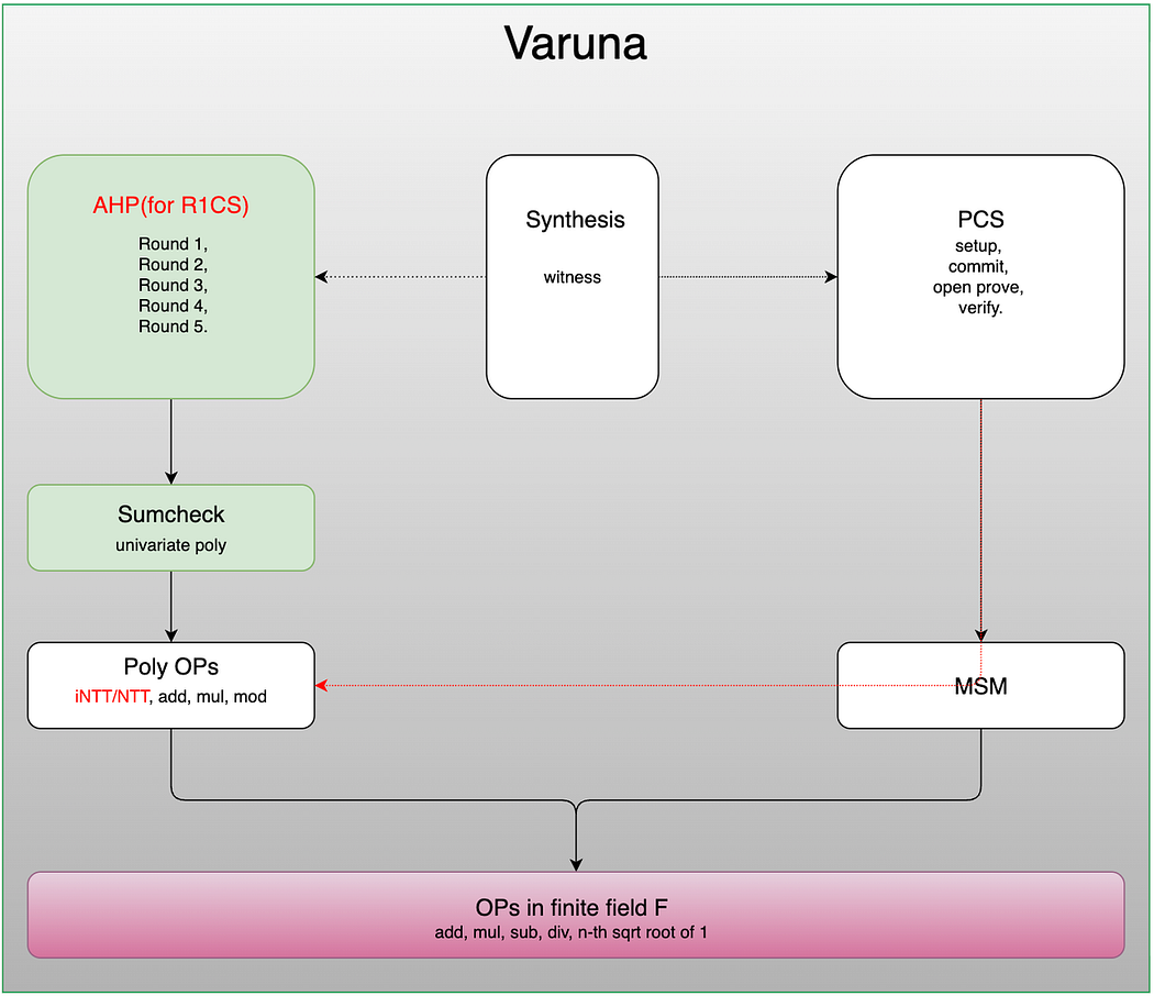
The Varuna algorithm primarily consists of three components: circuit synthesis, algebraic holographic proof, and polynomial commitment scheme. We will provide a detailed introduction and analysis of the algebraic holographic proof part of the Varuna ZKP algorithm (i.e., how constraints are proven through polynomial representation and computation), which is the most challenging part of Varuna.
This article will analyze and introduce the algorithm’s principles from a theoretical perspective, provide a simple mathematical reasoning process, and discuss the future evolution of Varuna in the context of the Aleo 2025 Roadmap.

As shown in the figure below, this article will focus on the left part of the diagram, namely the algebraic holographic proof (where “holographic” refers to the small number of queries required in the proof process). The circuit synthesis and polynomial commitment scheme, while logically somewhat complex, are similar to those in other proof systems.

The following text will explain the problem that Varuna proves, providing rigorous definitions of the terms used, and then analyzing in detail the five rounds introduced to address this problem (with Rounds 3 and 4 being more complex, while the other rounds are simpler). Due to space constraints, for the mathematical foundations involved, we will only briefly explain the concepts and theorems, without providing detailed descriptions or proofs, and encourage readers to refer to any abstract algebra textbook they find interesting.

3. R1CS Problem and Definitions

The purpose of the Varuna algorithm is to prove that the execution of a program (written in the Leo language, assuming a single program for now; the process for proving multiple programs will be discussed later) is correct. To achieve this, Varuna first executes the program and, based on the types of computations and intermediate results during execution, constructs three matrices A, B, C, and a vector z. This reduces the problem of proving the correctness of program execution to proving that these three matrices and the vector z satisfy certain constraints. We provide the following definition:

Definition 3.1: R1CS Problem
For given matrices A, B, C, and vector z, the R1CS (Rank-1 Constraint System) refers to proving that the following equation holds:

matrix A: An (m, n) dimension matrix over a finite field F (i.e., the elements of the matrix belong to F, not the real numbers). A finite field is a set in which the four basic arithmetic operations (addition, subtraction, multiplication, and division) can be performed, and the number of elements in the set is finite (for a rigorous definition, refer to textbooks).
matrix B, C: Defined similarly to A, but as distinct matrices, with all three matrices having the same dimensions.
z: An n-dimensional column vector in the finite field, where z includes the public inputs of the program and the witness (i.e., public inputs and intermediate results of program execution), such as z = (x, w).
Az: Denotes standard matrix-vector multiplication, resulting in a column vector a_z. Similarly, b_z and c_z are defined.
The product of Az and Bz: Represents the Hadamard product between column vectors, i.e., element-wise multiplication of corresponding elements in the two vectors.

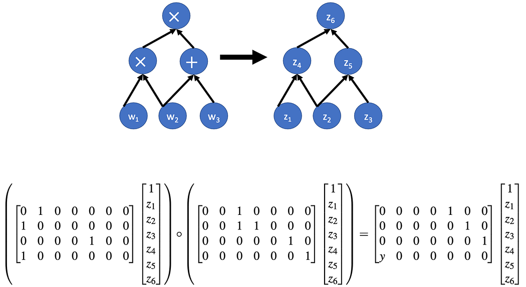
As shown in the simple example in the figure below, this illustrates how arithmetic operations of instructions are converted into an R1CS problem. Note that each row of the matrix corresponds to a constraint, and the constraint holds if and only if the corresponding instruction’s computation is correct.

Source: Proofs, Arguments and Zero Knowledge by Justin Thaler

Lemma 3.2: Sum-check

For a given polynomial f(Y) over a finite field F (i.e., the coefficients of the polynomial belong to F), the sum of f over a cyclic group C (a non-zero multiplicative subgroup, slightly abuse notation with C in R1CS, but easy to get the difference) in F equals σ, if and only if there exist polynomials h(Y) and g(Y) over F such that the following equation holds:

σ: An element in F.
C: A subgroup of the multiplicative group formed by all non-zero elements in F under multiplication. Group, a set with a defined “multiplication” operation. Notably, any multiplicative subgroup in a finite field is a cyclic group, meaning every element in the group is an integer power of some element. This is crucial because many algorithms in zero-knowledge proofs (especially Varuna) rely on the simple structure of cyclic groups.
|C|: The number of elements in the cyclic group C. Since F is finite, C is necessarily finite.
vC(Y): The vanishing polynomial over the cyclic group C, i.e., a polynomial that evaluates to zero at every element of C. Other vanishing polynomials over cyclic groups can be defined similarly.

For ease of discussion in the following sections, we assume that the row indices of the three matrices in R1CS, such as those in A, are treated as a function from a cyclic subgroup R of F to F. We call this cyclic subgroup R the constraint domain (i.e., constraint_domain in the code). The cyclic subgroup C corresponding to the column indices is called the variable domain (i.e., variable_domain in the code). Based on the context, it is easy to distinguish whether C refers to the matrix in R1CS or the variable domain, avoiding symbol confusion.
Clearly, z should be treated as a function from R to F , and the public inputs of the program to be proven (i.e., public_input in the code) are treated as a function on a subgroup H0 of R, which we call the input domain (i.e., input_domain in the code).
Additionally, as seen in the R1CS example above, many elements in the three matrices are zero. To save memory and computation, all non-zero elements in each matrix are sorted in the order of their appearance, and the subgroup K corresponding to the indices of this sorting is called the non-zero parameter domain (i.e., nonzero_domain in the code).

4. Round 1: Generating the Witness Shift Polynomial and Random Polynomial

4.1. Computing the Witness Shift Polynomial
The following polynomial is computed:

x: The public input of the program to be proven.
H0: The input domain, with its number of elements being the smallest power of 2 greater than or equal to the number of elements in the public input.
vH0(X): The vanishing polynomial over H0。
hat_x(X): The low-degree extension polynomial of the public input x, obtained using the function values of x on H0 via IFFT.
z’(X): The low-degree extension polynomial of the function z’, where z’ represents the public input and witness.

4.2. Generating the Random Mask Polynomial
The generation process is relatively simple, as shown in the following equation:

R3(X), R4(X): Polynomials with coefficients that are random elements in F, with R3(X) of degree 3 and R4(X) of degree 4.
vC(X): The vanishing polynomial over C (in the code, this corresponds to the maximum variable domain).

Why is the mask polynomial needed?
It is used in Round 3 to achieve zero-knowledge properties.

4.3. Prove process

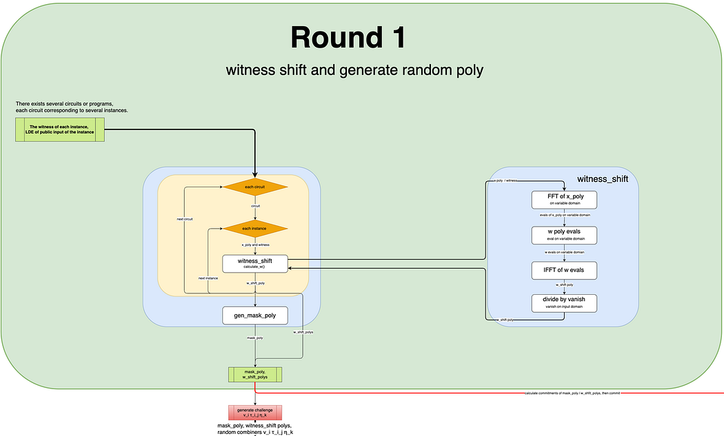
The figure below illustrates the computation process for Round 1. Note that the figure involves iterating over circuits and multiple instances of each circuit. This is because Varuna supports what is known as batch proving, where multiple circuits and their respective multiple executions are proven together, generating only a single proof.

5. Round 2, row check

5.1 Prove Principle
The goal is to prove the following:

a_z = Az, the product of matrix A and column vector z = (x, w), with similar definitions for b_z and c_z
The multiplication on the left-hand side is element-wise multiplication, not a vector inner product.
the equation being proven consists of m equations, corresponding to m constraints. If the program is executed correctly, these m equations hold.

How to prove it? It’s straightforward.

1. Use IFFT to compute the low-degree extension polynomials of a_z, b_z and c_z, obtaining hat_az(X), hat_bz(X) and hat_cz(X).

2. (Eq. 5) holds, meaning every constraint in the R1CS is satisfied, if and only if for any element x in R, x is a root for the equation: hat_az(X)·hat_bz(X) — hat_cz(X) = 0.

3. The statement in step 2 holds if and only if the vanishing polynomial v_R(V) over ( R ) divides hat_az(X)·hat_bz(X) — hat_cz(X). That is, there exists a polynomial h0(X) on F such that:

4. (Eq. 6) holding is almost equivalent to the following equation holding, in which α∈F\R is a random challenge value from:

5. The purpose of Round 2 is to compute h0(X), calculate its commitment value, and submit it.

6. When the verifier receives the proof for verification, they need to check that (Eq. 7) holds.

5.2 Prove process

The specific proof process for Round 2 is illustrated in the figure below:

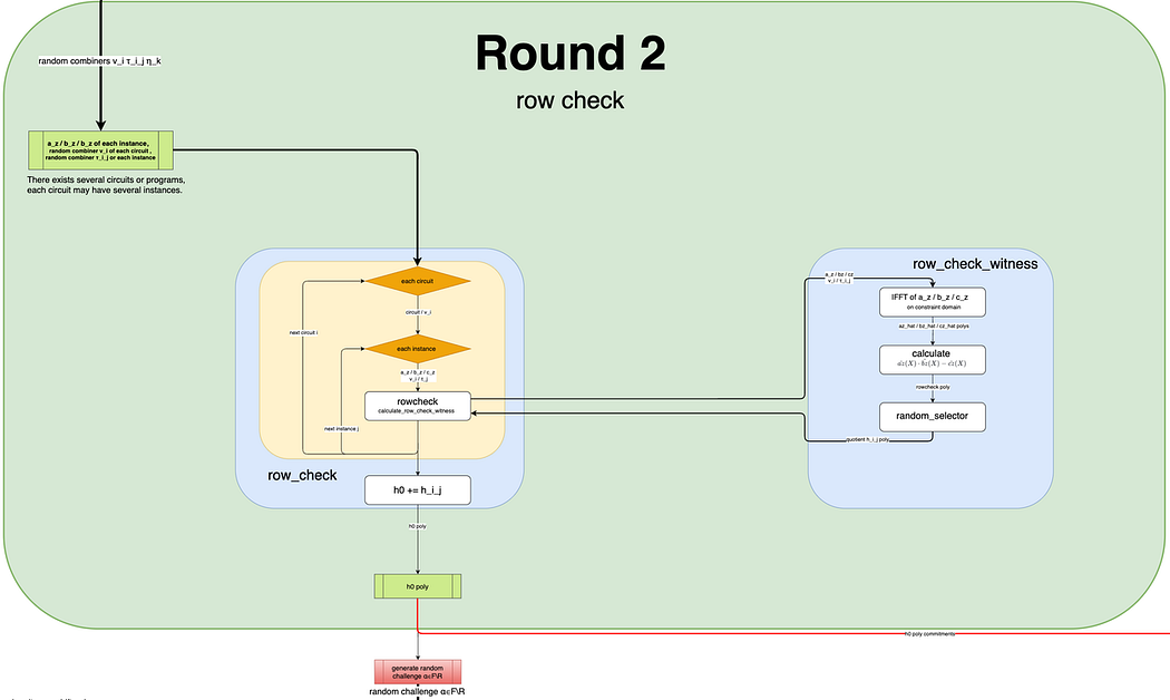
Note that in Round 2, the process iterates over multiple circuits and multiple instances of each circuit, computing the row_check_witness.

The most important feature of Varuna is its support for batch proving, which involves proving multiple circuits and their multiple instances together, generating a single proof.

Since there are multiple circuits, each potentially with multiple instances, a naive implementation would require computing the h0(X) polynomial for each instance of each circuit, calculating its commitment value, and submitting it. However, this approach would result in many commitment values being submitted, leading to a large proof size.

Instead, we aim to combine all quotient polynomials from multiple circuits and instances into a single polynomial and submit its commitment value. This is achieved by computing the following expression, derived through easy mathematical reasoning.

R: The largest constraint domain.
Ri: The constraint domain of the i-th circuit.
vRi(X): The vanishing polynomial over.

6. Round 3, linear check

6.1 prove principle
Linear check is to compute and prove that the matrix-vector multiplication is correct, i.e., compute and prove that the following equation holds:

M ∈ {A, B, C}, with a_z denoting the product of matrix A and vector z = (x, w), and similarly for b_z and c_z.

Why is this necessary?

Get Computation Frontier’s stories in your inbox

Join Medium for free to get updates from this writer.Subscribe

1. The R1CS itself requires proving this equation.

2. During verification in Round 2, the verifier needs to compute:

However, the verifier cannot directly compute this because they do not have M (which may be very large) or z. Thus, they rely on the prover.
Note that (Eq. 11) holding is almost equivalent to (Eq. 10) holding, so we only need to compute and prove (Eq. 11).

How to prove it?
For ease of explanation, we first assume there is only one circuit. The intuitive understanding of the proof process is as follows:

1. Leverage the sum-check protocol for a univariate polynomial over the cyclic group ( C ). Sum-check Lemma: As stated in Definition 3.2, for a polynomial ( f(Y) ), the sum over the cyclic group C equals σ, if and only if there exist polynomials h(Y) and g(Y) such that:

2. Note that the matrix-vector multiplication is essentially a summation.

3. The key to the proof is computing f(Y) = hatM(α, Y) · z(Y), where hatM(α, Y) is the low-degree extension of M as a bivariate polynomial.

4. To compute f(Y), consider the Lagrange basis expansion of hatM(X, Y):

R: The constraint domain, i.e., the domain of the row indices of M.
C: The variable domain, i.e., the domain of the column indices of M.
K : The cyclic subgroup corresponding to the indices obtained by sorting all non-zero elements of matrix Min their order of appearance, i.e., the non-zero domain in the code.
valM(κ): The function that treats all non-zero elements of M as a function over K, with hat_valM(Z) as its low-degree extension polynomial.
rowM(κ): The function that treats the row indices of all non-zero elements of M as a function over K, with hat_rowM(Z) as its low-degree extension polynomial.
colM(κ): Defined similarly to rowM(κ).
L_rowM(κ)_R(X): The Lagrange basis function corresponding to the rowM(κ)-th element over R, and similarly for L_colM(κ)_C(Y)

5. Using the low-degree extension of M(Eq.13), we can easily construct f(Y).

6. Then, applying the sum-check lemma, (Eq. 11) holding is almost equivalent to the following equation holding, where β is a random challenge value in F\C:

7. The purpose of Round 3 is to compute h(Y) and g(Y), submit them, and ensure zero-knowledge properties.

8. The verifier, during verification, needs to check that (Eq. 14) holds.

6.2 Prove process

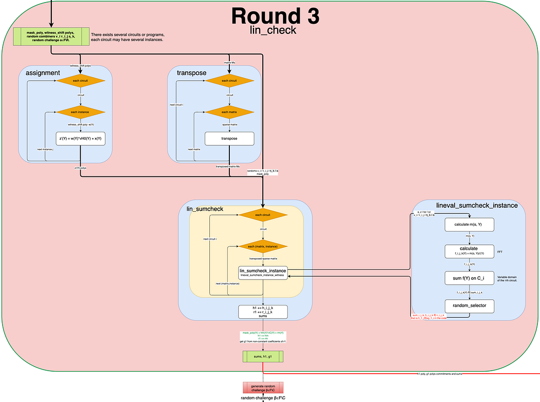
Additionally, note that in Round 3, the process iterates over multiple circuits and multiple instances of each circuit. Similar to the prove process in Round 2, for multiple circuits and instances, we aim to combine all quotient polynomials h(Y) and remainder polynomials r(Y) into a single polynomial, i.e., compute h1(Y) and r1(Y) in the following equations and submit their commitment values:

C : The largest variable domain.
Ci: The variable domain of the i-th circuit.
vC(Y): The vanishing polynomial over C.
h’_ijk(Y) and r’_ijk(Y) must satisfy the following equation:

7. Round 4, rational check

7.1 Prove principle

Compute and prove the evaluation of the bivariate matrix polynomial

M ∈ {A, B, C}.
hatM(X, Y): The low-degree extension polynomial of M, as noted in (Eq. 13).
α: A random challenge value from F\R.
β: A random challenge value from F\C.

Why is this necessary?

1. In Round 3, the verifier needs to compute hatM(α, β) for the final check, but cannot do so directly (due to high computational cost). Thus, the prover must compute and prove it.

2. Directly using the bivariate polynomial obtained from the Lagrange expansion of the matrix for the proof would be computationally expensive. Therefore, a derivative polynomial basis is introduced. Below are the Lagrange basis function expansion and the derivative polynomial basis function expansion:

dR(X, Y) = [vR(X) — vR(Y)] / (X — Y).
R: The constraint domain.
C: The variable domain.
K: The non-zero parameter domain.

How to prove (Eq. 17)?
For ease of explanation, we first assume there is only one circuit.

1. Using the definition of the quotient polynomial, simplify (Eq. 18), obtain the following expression:

2. Define the following polynomial r(Z):

Then, (Eq. 17) holds if and only if the sum of the rational polynomial r(Z) over K equals ω.

3. The statement in step 2 holds if and only if there exist polynomials h4(Z) and gM(Z) such that the following equation holds:

4. The purpose of Round 4 is to compute ω, hM(Z), gM(Z), a(Z), b(Z) from the above equation, and submit them (for polynomials, compute their commitments).

7.2 prove process

Based on the above description, we can obtain the proof process for Round 4 as shown in the figure below:

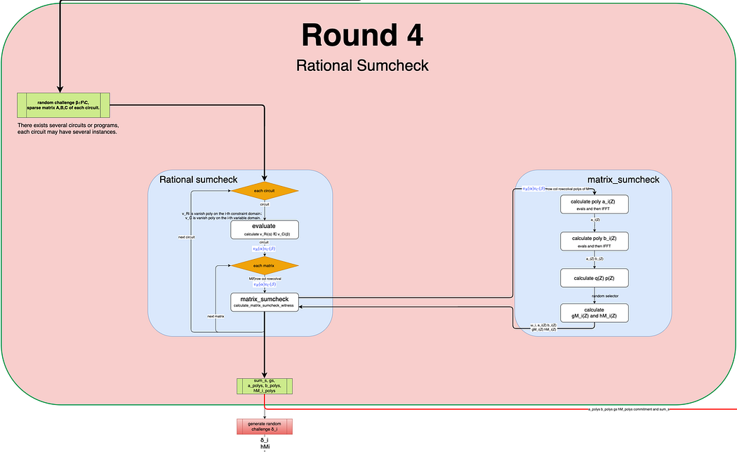
Similar to the approaches in Round 2 and Round 3, all hM_i(Z) polynomials are combined (using random selection, but the combiner is obtained later and accumulated in Round 5).

8. Round 5

The process for Round 5 is relatively simple, only requiring the completion of the following computations:

9. Summary

In summary, the proof process for the algebraic holographic part of Varuna primarily consists of the following five rounds:

Round 1: Preparation for the proof, generating the witness_shift polynomial and the random polynomial mask(X), used to achieve zero-knowledge ZK.

Round 2: Row check, proving that each row constraint in the R1CS holds.

Round 3: Linear check, computing and proving that the matrix-vector multiplication is correct, while also supporting Round 2.

Round 4: Rational check, supporting Round 3, computing and proving the evaluation of the low-degree extension polynomial of matrix M at (α, β): ω = hatM(α, β).

Round 5: Randomly combining the quotient polynomials from Round 4 and computing their commitment values, supporting Round 4.