
Binius Proof System, PCS
Binary-tower fields, small memory footprint, and the PCS at the core of Binius.
TL;DR
Binius Proof System is ZK proof system based on Binary Tower, which offers small memory footprint and high efficient field computation. We analysis the PCS in the Binius — which is an essential component to any ZK proof system, in an intuitive but strict manner. We introduce the motivations to the PCS used in Binius, then analysis commitment, and ring switch, Multi-variate Sumcheck protocol, FRI which are used to open prove of the commitment.
1. Definition and Motivation
PCS Commit
The polynomial t(X) corresponding to the trace or witness contains sensitive information and is relatively large in size (due to its high degree). To achieve ZKSNARK in the proof process, we cannot directly include the polynomial (e.g., its coefficients) in the proof. Instead, the polynomial’s coefficients are compressed to produce a smaller value (e.g., a 256-bit hash).
This value is called the commitment value, and the process is known as the commit computation.
For example, in RISC0, for a given polynomial ( t ), NTT is performed on the commitment domain to obtain the leaves of a Merkle Tree, which is then constructed, with the tree’s root serving as the commitment value.
PCS Open Proof
During the proof process, it is necessary to evaluate the polynomial t at a specific challenge value r. The prover needs to compute the function value β = t(α) of the polynomial t and prove that this computation is honest (i.e., to avoid using a forged polynomial).
This process is called the PCS open proof. The commit and open proof are the two most critical steps in PCS. Generally, the commit step is straightforward, while the open proof is more complex.
In RISC0 V2, the PCS is based on Merkle Tree (Hash) + FRI (RS code), while in Varuna, the PCS is based on KZK10 MSM. In Binius, the PCS is based on Merkle Tree (Hash) + Sumcheck + FRI (RS code).
Notably, the use of FRI differs significantly between the two. In RISC0, FRI is used for low-degree testing (combined with quotient polynomials) to perform the open proof, whereas in Binius, FRI is used for the open proof of large-domain polynomials (large and small domain polynomials will be discussed later). Additionally, the construction of RS codes is entirely different.
This is Binius’s primary contribution. Its PCS is based on Merkle Tree (Hash: Groestl256), Multi-Variate Sumcheck, and FRI (RS code). Merkle Tree and Hash are relatively straightforward, while the other concepts are more complex, as discussed below.
RS Code
RS code refers to a set of codewords, where a “codeword” is defined as the set of all function values of a polynomial t evaluated on a set S. The process of computing the codeword for a polynomial t is called encoding, with the polynomial t referred to as the message. We assume the t is a polynomial on finite field F.
For example, in RISC0, the codeword of polynomial t consists of all its function values on the commitment domain (that is set S ). Computing these values using multiplicative FFT requires that the commitment domain forms a cyclic multiplicative group with order is a power of 2 (in the complex field, FFT is feasible because there exist cyclic multiplicative groups of any order on the unit circle in the complex plane). Since all computations occur in a finite field F, it is required that F contains such a multiplicative subgroup.
Additionally, for RS codes, the codeword length, i.e., the size of the commitment domain H, must satisfy |H| > deg(t)+1 = trace length , as RS codes are error-correcting codes (errors in the information can be easily detected, corresponding to soundness), which necessitates the introduction of redundancy.
Additive NTT
Defined as follows: given the coefficients of a polynomial t: t_{0}, …, t_{2^l-1}, compute the function values of another univariate polynomial P over the hypercube B_{l+R}.

In which,
- B_l is the additive subgroup (corresponding to the trace domain in RISC0),
- B_{l+R} is the additive subgroup containing B_l, corresponding to the commitment domain in R0, though in practice it is a coset,
- R is the blowup factor, which is 2 in R0 and 1 in Binius,
- X_j(X) is the basis function of the polynomial vector space over F, completely different from the standard basis functions 1, X, X², …, For its strict definition, refer to this.
MLE
Multi-Linear Extension: For a given function t:B_l → F, its multi-linear extension is a polynomial function tilde_t(X_0,…,X_{l−1}) that satisfies:
- tilde_t is linear in each variable X_j, i.e., the degree of tilde_t with respect to any variable X_j is at most 1, making tilde_t multi-linear;
- The function values of tilde_t on the hypercube B_l are equal to the function values of t, tilde_t is an extension of t.
As shown in Equation (Eq. 2) for tilde_t, the polynomial tilde_eq is precisely the Lagrange basis for the multivariate polynomial (where the set formed by the MLE of all l-variables is viewed as a 2^l-dimensional vector space).


Why MLE?
In RISC0, the algebraic proof relies on the divisibility between the constraint polynomial and the vanishing polynomial on the evaluation domain. However, in a binary field, there is no multiplicative subgroup, and the vanishing polynomial lacks a simple or efficient computation method.
To address this, Binius adopts a Zero Check based on multivariate polynomials for the proof. The Zero Check is proven using the multivariate polynomial Sumcheck protocol (which we will introduce later). The trace is treated as the simplest case of a multivariate polynomial, i.e., a multilinear polynomial, obtained through MLE.
(Why not use the univariate polynomial Sumcheck from Varuna for the proof? For the same reason: the absence of a multiplicative subgroup.)
2. Binius PCS Commitment
All computations in Binius are performed in a binary field, such as F2 ~ F2⁷, which offers the advantages of efficient computation and reduced memory usage.
However, to achieve these benefits while adhering to the constraints of Reed-Solomon (RS) codes, conflicts arise. The design of the Polynomial Commitment Scheme (PCS) in Binius is primarily aimed at resolving these conflicts.
- Conflict 1: In a binary field tower, there is no multiplicative subgroup of a power of 2 (due to Lagrange’s theorem), so multiplicative FFT cannot be used. However, additive subgroups exist in the binary field, enabling the use of additive NTT.
- Conflict 2: In the coefficient field (small field) of the polynomial t, there is no sufficiently large subgroup to serve as the commitment domain for RS codes. RS codes require the commitment domain size |H| > deg(t)+1 = trace length, but we want the trace length to be sufficiently large (e.g., segment size), while keeping the memory usage of t minimal, i.e., preferring a small coefficient field F. Additionally, H must be a subset of the finite field F(since all encoding computations occur in F). For example, if the finite field F2⁴ and the segment size or |H| is 2¹⁹, no subset of F2⁴ can serve as H, since |F2⁴| = 2¹⁶ < 2¹⁹.
For Conflict 2, a naive approach would be to directly embed all coefficients of t into a larger field (e.g. F2⁷), but this increases memory usage and computational overhead (i.e., embedding overhead).
Binius addresses this by using a packing technique, where multiple adjacent coefficients of t are packed into a single element in the larger field. For example, if the polynomial t on F2⁴ has coefficients [t0, t1,… ], where each element has a bit width of 16 bits, Binius packs eight adjacent elements into a single element in F2⁷, resulting in a polynomial t′ on F2⁷, as illustrated below:

Subsequently, using RScode to encode t′ which is a polynomial over the larger field, resolving Conflict 2. Then, the Merkle Tree root node of t′ is computed as the commitment value. The PCS in Binius is also referred to as the small-field PCS.
3. Ring-Switch
As previously mentioned, to address the issue of the coefficient field of polynomial t lacking a sufficiently large commitment domain when using RS codes, Binius introduces the packing technique. This involves packing adjacent coefficients of t into a polynomial t′ over a larger field, followed by computing the Merkle Tree root node of t′ as the commitment value.
However, this introduces another challenge: while the Merkle Tree commitment is made using t′, the proof opening requires computing the function values of the small-field polynomial t(failing to address this could lead to security issues).
To resolve this, Binius employs Ring-Switch and Sumcheck to reduce the problem of opening the commitment of t to opening the commitment of t′, where the commitment opening proof for t′ is achieved through FRI folding and Merkle Tree queries.
The PCS in Binius is also referred to as the small-field PCS. The purpose of Ring-Switch is to reduce the opening proof of the small-field PCS to that of the large-field PCS, which is somewhat complex. We attempt to explain as follows:
Suppose the small-field MLE is t(X_0,…,X_{l−1}), and after packing, the resulting polynomial is t′(X_0,…,X_{l−κ}). We need to prove s = t(r_0,…,r_{l−1}), where:
- r_j are random challenge values from the large field (for security reasons, random challenge values are typically drawn from the large field, e.g., F2⁷);
- κ is the packing or extension coefficient. For example, if each coefficient of t is an element of F2⁴(bit width of 16 bits), and each coefficient of t′ is an element of F2⁷(bit width of 128 bits), then κ = log2(128/16) = 3.
For convenience, we denote the coefficient field of t as K, and the coefficient field of t as L, where L is an extension of K of degree 2^κ. Additionally, L is a 2^κ-dimensional vector space over K, with basis β_0,…,β_{2^κ−1}. We also denote l′=l−κl.
Note that our goal is to prove (Statement 1):

3.1 How to Prove (Statement 1)?
Note that by treating r_0,…,r_{κ−1} as variables and based on the definition of MLE, we can deduce:

Thus, we conclude that (Statement 1) holds if and only if (Statement 2) holds:

This is because, in the right-hand side of (Statement 2),
Get Computation Frontier’s stories in your inbox
Join Medium for free to get updates from this writer.Subscribe
v_0,…,v_{κ−1} traverse the hypercube B_κ. After receiving hat_s_v, the verifier can easily compute t(r_0,…,r_{l−1}) according to (Eq.1.1) and then determine whether s equals t(r_0,…,r_{l−1}). Thus, the problem reduces to proving (Statement 2).
3.2 How to Prove (Statement 2)?
We expand all hat_s_v∈L in terms of the basis β_0,…,β_{2^κ−1}, obtaining the following expression:

Additionally, note that by expanding the polynomial t(v_0,…,v_{κ−1}, X_κ,…,X_{l−1}) in terms of the Lagrange basis and evaluating it at r_κ,…,r_{l−1}, we obtain:

We conclude that (Statement 2) holds if and only if (Statement 3) holds:

In fact, we have used two methods to compute hat_s_v:
- On the left-hand side of (Statement 2), the hat_s_v is expanded in terms of the basis for vector space of L over K, according to (Eq. 2.1).
- On the right-hand side of (Statement 2), the polynomial is expanded in terms of the Lagrange basis and then evaluated, according to (Eq. 2.2)
Thus, the problem reduces to proving (Statement 3).
3.3 How to Prove (Statement 3)?
To connect with t′, as we aim to reduce the small-field opening proof to the large-field opening proof, we can attempt to express β_u in terms of β_v Noting that v appears in t in (Statement 3), we expand the function values of the hat_eq polynomial value:

By substituting (Eq. 3.1) into (Statement 3) and simplifying, and leveraging the linear independence of the basis in the vector space, we conclude that (Statement 3) holds if and only if (Statement 4) holds:

Thus, the problem reduces to proving (Statement 4).
3.4 How to Prove (Statement 4)?
By multiplying both sides by β_v and simplifying, we conclude that (Statement 4) holds if and only if (Statement 5) holds:

Where hat_s_u is defined as (Eq. 4.1):

Note that u in (Eq. 4.1) comes from the right-hand side of (Statement 4), which originates from (Eq. 3.1), and u in hat_s_u must match u in A_{w,u}.
Thus, the problem reduces to proving (Statement 5).
3.5 How to Prove (Statement 5)?
Since (Statement 5) is a standard Multi Sumcheck equation, it can be proven using the Multi Sumcheck Protocol. However, we aim to prove (Statement 5) holds for all u∈B_κ, batching them together to reduce the proof size. To this end, we have that (Statement 5) is almost equivalent to (Statement 6):

(Statement 6) can be proven using Multi Sumcheck. (Why? After replacing r′′ with κ variables on both sides of (Statement 6), both sides are MLEs. If (Statement 5) holds, (Statement 6) must hold; and if two MLEs are equal at a randomly chosen point, then (Statement 5) holds with overwhelming probability.)
3.6 Summary:
To prove (Statement 1):
Using fewer challenge values, (Statement 1) is equivalent to (Statement 2):
By computing hat_s_v using two different basis expansion methods, (Statement 1) is equivalent to (Statement 3):
To connect with t′, eliminate β_u, (Statement 3) is equivalent to (Statement 4):
Multiplying by β_v and simplifying, (Statement 4) is equivalent to (Statement 5):
Batching the Sumcheck proof, (Statement 5) is almost equivalent to (Statement 6):
Finally, we define the polynomial ( h ):

where A is given by (Eq. 6.2):

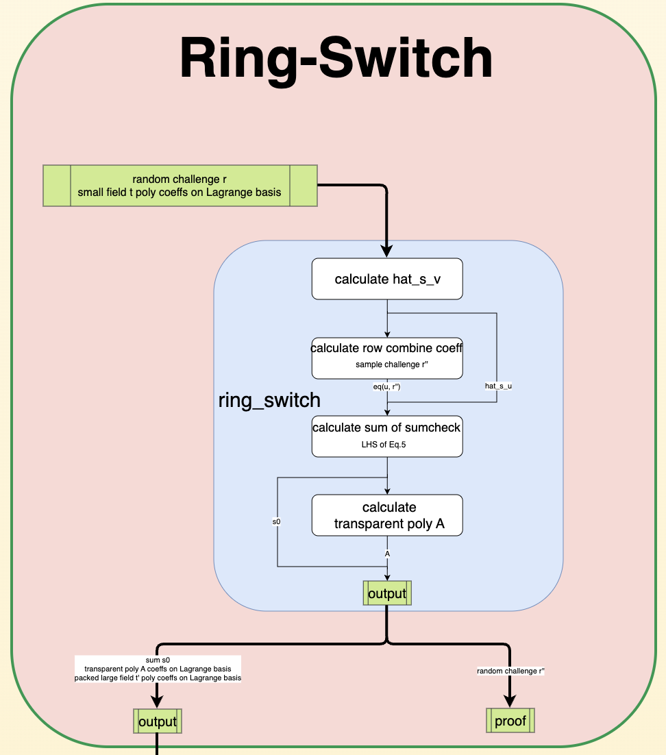
The purpose of Ring-Switch is to compute the polynomial h, the left-hand side of (Statement 6) s0, for subsequent Sumcheck proof and FRI. The specific algorithm flow is shown in the figure below:
4. Sumcheck FRI
Sumcheck Protocol
The purpose of the Sumcheck protocol is to prove the following equation holds:

where h is defined as in (Eq. 6.1). The prover needs to demonstrate that this equation holds without revealing the coefficients of h. From the equation above, it can be seen that the right-hand side is effectively a sum of the function values of the polynomial over all vertices of the “hypercube,” i.e., Sumcheck.
Prover:
There are a total of l’ rounds, and the proof proceeds as follows:
For j=round_1, …, round_l′:
A. The prover computes the coefficients of the univariate polynomial:

B. The prover appends the coefficients of H_j to the current transcript.
C. The prover uses the generated transcript as input to produce a random challenge value r′_j.
D. The prover computes the coefficients of the multivariate polynomial h(r′_1,…,r′_j, X_{j+1},…,X_{l′}).
Verifier:
Upon receiving the transcript, the verifier locates the section corresponding to the Sumcheck and extracts each univariate polynomial H_j.
For j=round 1, …, round_l′:
The verifier checks if H_j(0)+H_j(1) = H_{j−1}(r′_{j−1}).
— If this holds for all j, the verifier accepts the Sumcheck as correct.
— Otherwise, the verifier considers the Sumcheck incorrect.
Additionally, the verifier checks if H_l′(r′_l′) == h(r′_1,…,r′_l′).
Note that in the final step, the verifier needs to check
H_l′(r′_l′) == h(r′_1,…,r′_l′) = A(r’_1, …, r’_l’) * t′(r’_1, …, r’_l’). Here, the verifier can computeH_l′(r′_l′) and A(r′_1, …, r′_l′) independently (why? refer to the definition in Eq. 6.2, which involves the hat_eq polynomial). However, t′(r′_1, …, r′_l′) cannot be computed by the verifier (to ensure zero-knowledge, the verifier does not have access to it).
The prover use FRI to compute and prove t′(r′_1, …, r′_l′). How is this proven? After FRI folding, the RS code of t′ becomes a constant function, and this constant is exactly t′(r′_1,…,r′_l′)(why? refer to the this). Additionally, a Merkle Tree path proof is required to ensure the folding process is correct.
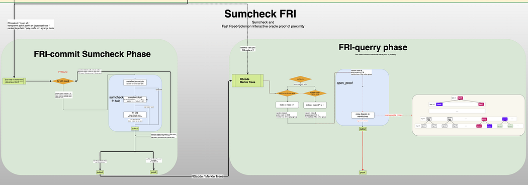
The specific algorithm flow is shown in the figure below:
5. Conclusion
The Binius Proof System’s PCS is a sophisticated and innovative scheme that optimizes for binary fields, offering a balance of efficiency, security, and practicality. By addressing the limitations of binary fields through techniques like additive NTT, MLE, and Ring-Switch, Binius provides a robust framework for zero-knowledge proofs, particularly in scenarios where computational resources are limited. Its design not only enhances performance but also sets a new standard for ZK proof systems in constrained environments. Especially, it’s friendly to hardware such as FPGA or ASIC, thus it might be further accelerated.