
Finite Field Arithmetic Optimization
Novel field-multiplication algorithms worth at least 20% on the inner loop.
TLDR
The finite field arithmetic operations are essential in ZKP proof systems, we introduce some simple novel field computation algorithms, result in at least 20% performance improvement of multiplication in extension field K, and 30% improvement of Montgomery transformation from integer to Montgomery representation in the base field F.
1. Goal
In many zero-knowledge proof systems (such as SP1 and RISC0), the majority of computations occur within finite fields, including finite field addition, multiplication, and division. Therefore, efficient finite field arithmetic operations are crucial for the performance of zero-knowledge proof systems. We will introduce some novel finite field computation algorithms and provide performance comparison data.
2. Finite Fields
A field is a set F equipped with two operations, referred to as “addition” and “multiplication”, denoted as + and ⋅ respectively, that satisfy the following conditions:
A. F forms an Abelian group under addition:
- There exists an additive identity element 0∈F.
- Every element in F has an additive inverse.
- Addition is associative and commutative.
B. F∖{0} forms an Abelian group under multiplication:
- There exists a multiplicative identity element 1∈F∖{0}.
- Every non-zero element in F has a multiplicative inverse.
- Multiplication is associative and commutative.
For example, the set of real numbers R, under standard addition and multiplication, forms the real number field R. A field F is called a finite field if it contains a finite number of elements.
A prime field Fp is defined as the set Fp={0,1,2,…,p−1}, where p is a prime number. Its operations are:
- Addition: a+b=(a+b) mod p (where the second “+” denotes integer addition, and mod is the modulo operation).
- Multiplication: a⋅b=(a×b) mod p (where × denotes integer multiplication).
A field extension K of a field F is a field such that F is a subfield of K (i.e., F⊆K, and the operations of K, when restricted to F, satisfy the field axioms). For example, the complex numbers C form an extension field of the real numbers R.
Since prime fields Fp are widely used in zero-knowledge proof systems, we focus on computations in Fp and their extension field K. Without loss of generality, we assume that:

Easy to know that polynomial X4+11 is irreducible in F[X], then the quotient ring F[X]/(X^4+11) forms a field and is an extension of F.
3. Operations in the Field F and Its Extension Field K
Operations in the field F typically include addition, subtraction, multiplication, and finding inverses, where addition and multiplication are the basic operations defined in the field F, while subtraction and inversion can be constructed from these basic operations. Similarly, operations in the extension field K can be derived from those in F, so we first focus on addition and multiplication in F.
Based on the definition of the prime field, addition in F is defined as a+b = (a+b) mod p. Note that 0≤a≤p−1, 0≤b≤p−1. When a+b is computed as integer addition, the result c=a+b satisfies 0≤c≤2p−2. Thus c mod p can be computed as: c mod p = if c<p then c ; otherwise c−p. This means that addition in F can be easily calculated using 1~2 integer addition/subtraction operations and one logical comparison.
Multiplication in F is defined as a⋅b=(a⋅b) mod p. Note that 0≤a⋅b≤(p−1)^2. When a⋅b is large, numerous subtraction operations are required to reduce a⋅b to an element in the field F. Alternatively, one division can be used, such as q = ⌊(a⋅b)/p⌋, and (a⋅b) mod p = (a⋅b)−(p⋅q). However, division operations require a significant number of cycles in hardware or GPU implementations. To address this issue, we introduce Montgomery reduction.
4. Montgomery Reduction
To reduce a given large integer to the range [0, p) without using division, Montgomery reduction bases on the following equation:
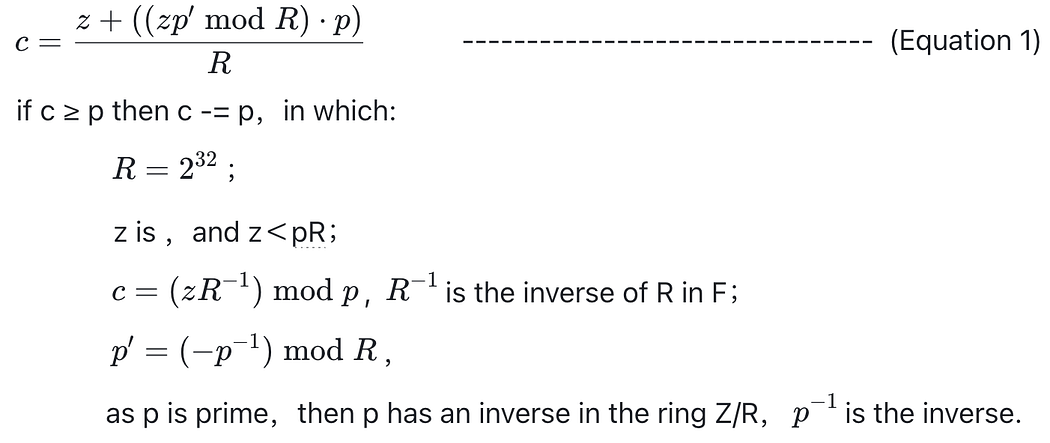
This equation clearly holds because, by considering the operations in the expression z + ((z⋅p′ mod R)⋅p) as multiplication and addition in the ring Z/RZ, there exists an integer k such that the following relationship is satisfied:

That is, the numerator in Equation (1) is a multiple of ( R ).
Get Computation Frontier’s stories in your inbox
Join Medium for free to get updates from this writer.Subscribe
Additionally, note that Rc = R(z⋅R_inv mod p). By treating the multiplication as an operation in the field F, we have:

For x∈[0,p), suppose tilde_x = xR mod p, with y and tilde_y defined similarly. According to the definition of the field F, the following equation holds:

From Equation (2), it can be seen that we can compute the product of tilde_x and tilde_y using Equation (1), i.e., Montgomery reduction and this equation. However, this requires first transforming x to tilde_x = xR mod p, which is computationally expensive. This transformation can be achieved, for example, via Mont(x,R2), where R2=(R⋅R) mod p, and R2 can be precomputed. In many proof systems, such a transformation typically needs to be performed only once, followed by numerous multiplication or division operations. Thus, Montgomery multiplication is an efficient method for multiplying elements.
Hereafter, we refer to this transformation as the Montgomery transformation, and tilde_x as its Montgomery representation.
5. Optimized Barrett Reduction
In many proof systems (such as SP1 and RISC0), when generating a trace, it is necessary to transform numerous integers in the range [0, 0xffffffff) into their Montgomery representation using the Montgomery transformation. However, the computational cost of the Montgomery transformation is relatively high. To address this, Barrett reduction can be introduced, as shown in the following equation:
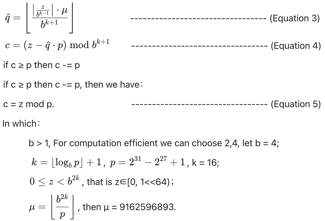
The correctness of Equation (5) or the proof of correctness for Barrett reduction can be found in Note 2.15 of Reference [1]. It suffices to note that, from this proof, it can be shown that: 0≤(z−hat_q⋅p) < 3p.
However, note that since μ>(1≪32), requires a u64 to represent μ. Additionally, since 0≤⌊z / b^(k−1)⌋< (1≪34), it also requires a u64 to represent. This results in one u64-u64 multiplication and one u64-u32 multiplication, which is computationally expensive. To address this, we can leverage the properties of μ and p to simplify the computation.

Additionally, Montgomery transformation is tilde_x = xR mod p, then let

Use Equation6 ~ Equation 8, we can change Equation 3 and Equation 4 to the following form:

Then the Optimized Barrett reduction just need one u32 multiplication, and other shift, add and subtraction, which are more efficient than multiplication operations.
6. Multiplication in the Extension Field K
We know that the elements in the extension field K are essentially a set of polynomials { r(X)+q(X)p(X) | q(X)∈F[X] }, where p(X) is an irreducible polynomial, such as p(X)=X^4 + 11 as defined above, with r(X)∈F[X] and its degree less than 4.
Thus, elements in K can be represented by their corresponding polynomial r(X), which can be expressed using 4 elements from the field F as the coefficients of the polynomial.
The multiplication operation in the extension field K consists of polynomial multiplication followed by a polynomial reduction with respect to p(X):

Then h(X) = (f(X) ⋅ g(X)) mod r(X) with coefficients:

From Equation (10), it can be seen that multiplication in the extension field K is implemented through the multiplication and addition of elements in the field F. Notably, this primarily involves the inner product of vectors, such as computing inn3=a0⋅b2+a1⋅b1+a2⋅b2. If computed naively using the multiplication and addition operations in the field F, multiple Montgomery reductions would be required (e.g., inn3 requires 3 reductions), with each reduction involving a significant computational cost:

Suppose we have already performed the Montgomery transformation on a0 using Optimized Barrett reduction, i.e., tilde_a0 = a0⋅R mod p, and similarly for tilde_a1, tilde_a2, tilde_b0, tilde_b1, tilde_b2. Then tilde_inn3 is:

From Equation (12), it can be seen that we only need to perform a single Montgomery reduction, which significantly improves the computational performance of the inner product. Consequently, the multiplication operation in the extension field K can be optimized.
7. Performance Comparison
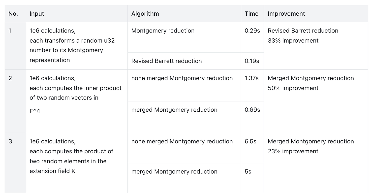
We implemented the following three simple algorithms in Python and collected performance data:
- Optimized Barrett reduction for Montgomery transformation;
- Merged Montgomery reduction in the computation of the inner product of two vectors.
- Merged Montgomery reduction for multiplication in the extension field K;
Test Platform: Mac M3, 16GB RAM, Python implementation.
8. Reference
1. Menezes, A. J., Vanstone, S. A., & Oorschot, P. C. V. (2004). Guide to elliptic curve cryptography. Springer.