RISC0 algorithm analysis, segment proof — Part1
RISC0 segment proofs, taken apart step by step.
TL;DR
RISC0 is a zkVM (zero knowledge Virtual Machine) based on the RISCV instruction set and STARK (Scalable Transparency Argument of Knowledge). RISC0 proof system consists with segment prove, recursion and STARK to SNARK proof. As segment prove occupies the largest amount of memory and computation, we focus on the analysis of segment prove process, including RAP, DEEP-ALI and FRI.
1. Purpose
RISC0 is a zkVM (zero knowledge Virtual Machine) based on the RISCV instruction set and STARK (Scalable Transparency Argument of Knowledge). We will introduce the overall proof process in RISC0 and focus on analyzing the segment prove, including its principle and the detailed proof process of the segment. Finally, we will compare the similarities, differences and advantages of RISC0 and other zkVMs.
2. RISC0 proof process
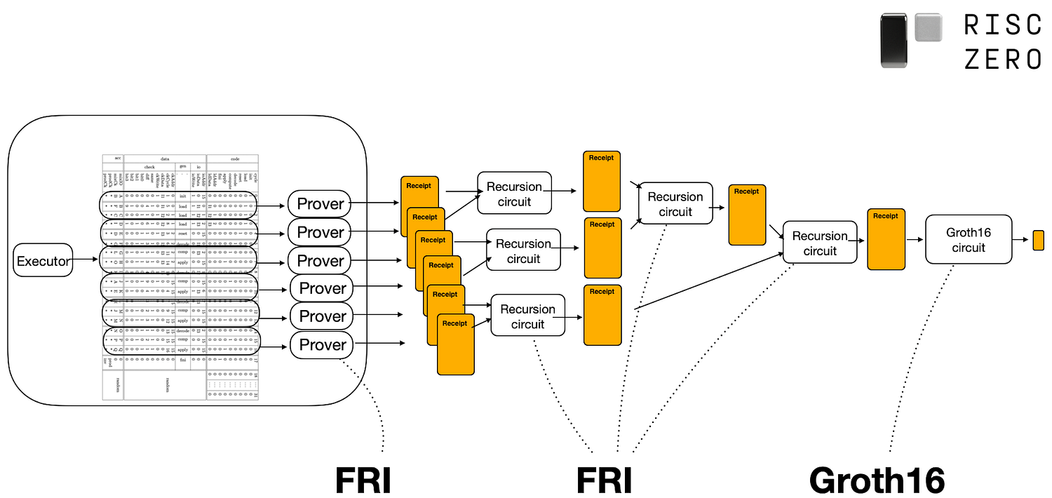
As shown in the figure above, for a program to be proved (composed of countless RISCV instructions, compiled by a high-level language such as rust) and its given input, RISC0 zkVM will execute the program and generate a proof file to prove that the program is executed correctly. At the same time, the proof file cannot contain any sensitive information, such as data generated during the execution process and private input. To this end, RISC0 zkVM will:
A. Execute the program, divide the program into multiple segments, and record the input and output of each segment;
B. Prove each segment and obtain the Receipt of each segment. This step is proved by the STARK/FRI protocol;
C. The Receipts obtained in the above steps are merged into one Receipt using recursive proving, so that proof files of the same length can be generated when proving programs of different sizes;
D. Convert the Receipt obtained by recursive proving into a snark proof through Groth16 to further reduce the proof size.
Segment prove occupies the largest amount of memory and computation. The following will analyze the detailed proof process of segment in detail.
3. Algebraic structure
Segment prove is a proof system based on the STARK protocol. To facilitate the description and understanding of segment prove, we need to introduce the algebraic structure required for the proof process, as shown in the figure below.
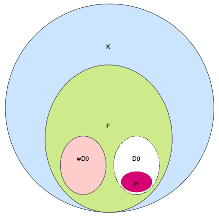
Among them,
F, is the finite prime field Fp, that is, F = Fp, p = 2³¹ — 2¹⁷ + 1, Fp is the Baby Bear prime field;
K, is the finite extension field of F, K = F[X]/(X⁴ + 11), that is, the quotient ring of the polynomial ring F[X] about the ideal (X⁴+11). It is easy to know that X⁴+11 is an irreducible polynomial on F, then the extension number of K relative to F is 4, and 1 element in K generally requires 4 elements in F to represent;
Why do we need the extension field K? To ensure security, the sample space where the challenge value is located must be large enough. The number of elements in F is only about 2³¹, while the number of elements in K is about 2¹²⁴.
D0, the cyclic subgroup of the multiplication group F/{0}, whose number of elements |D0|, such as 2²⁰;
H, the subgroup of D0, whose number of elements |H|, such as 2¹⁸, the trace domain; Why do we need the cyclic subgroup H? Because when interpolating and calculating a univariate high-order polynomial f(x), NTT/iNTT is used for efficient calculation, and the premise of NTT/iNTT is that x must be an element in the cyclic subgroup.
H is called the trace domain, which is important in STARK because most of the calculations and representations of all polynomials are performed on H.
wD0, the left coset of D0, w is the element in F that does not belong to D0, such as wD0 = {3*d | d∈D0}, called the commitment domain or evaluation domain. Why is the left coset wD0 needed? w is introduced to achieve zero knowledge. At the same time, polynomial calculations on the coset of the cyclic group only require simple transformation of the polynomial coefficients, and NTT/iNTT can also be used;
When performing segment proofs, it is often necessary to calculate or represent polynomials on the trace domain H and make polynomial commitments on the commitment domain wD0.
4 segment prove
The purpose of segment prove is to prove that the execution process of the sequential instruction stream is correct. This problem is converted into proving that the intermediate process (trace) of the execution satisfies the constraints of the polynomial equation group, and then converted into proving that the degree of a certain polynomial is relatively low (i.e., low-degree test problem). Finally, the FRI protocol is used to prove that the degree of the polynomial is relatively low. Segment prove mainly consists of set-up phase, RAP, DEEP-ALI, and FRI, as shown in the following figure:
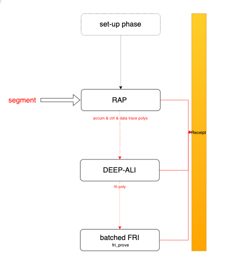
The set-up phase configures some proof parameters, such as the number of queries in the query phase of the FRI (Fast Reed-Solomon Interactive oracle proof of proximity) protocol, the maximum length of the trace, etc. At the same time, it will also generate the constraint polynomial between the traces (given in the form of source code, this part of the source code generates the function value of the constraint polynomial on the trace). It is worth noting that for a proven program, the set-up phase only needs to be executed once, and this process will not be discussed later.
RAP (Randomized Algebraic intermediate representation with Preprocessing) will execute the segment and record the intermediate data during the execution process (such as register values, memory access, etc.), with the purpose of calculating the trace polys, including ctrl & data & accumulate polys and commitments, which will be described in detail later.
DEEP-ALI (Domain Extending for Eliminating Pretenders — Algebraic Linking IOP) will calculate the check polynomial and fri polynomial. Check polynomial refers to the result obtained by substituting trace polynomials into the corresponding constraint polynomials and dividing them by the vanish polynomial. This is a key step in STARK, because proving that the execution process of a program is correct is equivalent to proving that the check polynomial is a polynomial and the degree of the polynomial is relatively low. In order to ensure that the calculation process of the check poly is correct, deep polynomials need to be calculated, and finally all deep polynomials are merged into one fri polynomial.
FRI (Fast Reed-Solomon Interactive oracle proof of proximity) aims to prove that the degree of the fri polynomial is less than or equal to the trace domain size. Below, we will introduce its process in detail.
5 RAP
The purpose of RAP is to calculate the control and data polynomial groups, which represent the values of the data register and control register during the segment execution process. In addition, in order to prove the correctness and range check of memory access behavior, a new set of polynomials needs to be generated: the accumulate polynomial group, which is used for permutation argument and lookup argument.
In addition, the merkle tree needs to be used to calculate the polynomial commitment values of the control & data & accumulate polynomial groups respectively.
Get Computation Frontier’s stories in your inbox
Join Medium for free to get updates from this writer.Subscribe
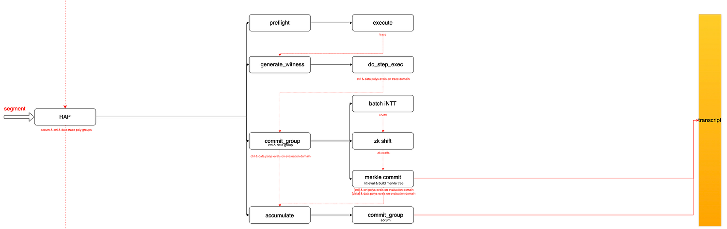
As shown in Figure 4, RAP consists of the following steps:
5.1 preflight/execute, sequentially execute the instructions in the segment, record the register address and value accessed by each instruction as raw_trace, and note that the data type is uint32;
5.2 generate_witness, convert the data in raw_trace into elements in F, calculate the values of all registers in each cycle according to raw_trace, and thus obtain a 2D matrix. Any row represents all register values in a certain cycle, and any column represents the value of a control or data register in all cycles. At the same time, the column is regarded as a function value of a control or data polynomial in the trace domain H, so the number of cycles must be less than or equal to the number of elements in H |H|. If the number of cycles is less than |H|, fill the missing rows of the matrix with 0.
5.3 For the control & data polynomial group (each polynomial is represented by a function value on H), calculate the commitment value of the polynomial:
5.3.1 iNNT calculates the coefficient of each polynomial, noting that the coefficient length of each polynomial is |H|;
5.3.2 Multiply the coefficient of each polynomial by 3^i, such as the coefficient of the nth polynomial is cn_0, …, cn_i, …, then cn_i = cn_i*3^i;
5.3.3 NTT calculates the function value of each polynomial on the commitment domain 3*D0;
5.3.4 Calculate the merkle tree for the function value of the control and data polynomial groups on the commitment domain,
then we will get 2 merkle trees, and the root node of the merkle tree is the commitment value.
5.4 For control & data polynomials (expressed by function values on H), in order to ensure the legality and range check of memory access, it is necessary to introduce the polynomials required by permutation constraints and lookup constraints, namely accumulation polynomials. To this end, it is necessary to:
5.4.1 Generate a random challenge value in the extended domain K for each permutation constraint and lookup constraint based on the commitment value of the existing control and data polynomial groups;
5.4.2 Calculate the polynomial corresponding to each permutation and lookup constraint (expressed by function values on H), which are collectively called accumulation polynomial groups;
5.4.3 Similar to the operation in 5.3, for the accumulation polynomial group, calculate its commitment value.
6. DEEP-ALI
For the convenience of description, we call all polynomials in the control polynomial group, data polynomial group, and accumulation polynomial group trace polynomials, and all function values of all trace polynomials on the trace domain H are called traces.
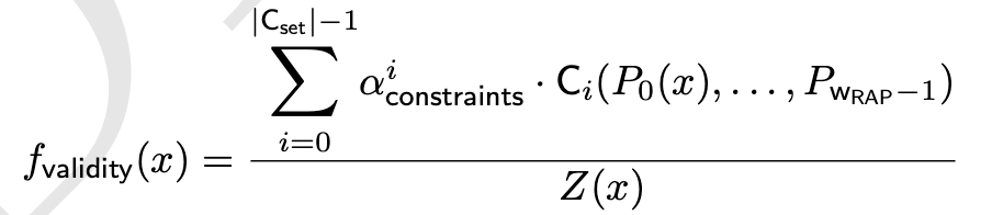
Our goal is to prove the correctness of the execution of instructions in the segment. This problem is reduced to a set of constraints (expressed as a set of multivariate polynomial equations) that must be satisfied between certain elements in the trace, and the establishment of this problem is equivalent to the constraint polynomial being able to divide the vanish polynomial on the trace domain H. DEEP-ALI will take the quotient of the constraint polynomial and the vanish polynomial to obtain the check polynomial and calculate its commitment value. In addition, to ensure that the check polynomial is calculated correctly, the DEEP polynomial will be calculated, and finally all the DEEP polynomials will be combined to obtain the FRI polynomial.
The definition of the check polynomial is as follows:
Among them,
α_constriants, is a random challenge value, belonging to the extended domain K;
Ci, is a constrained multivariate polynomial;
P0(X), …, is a trace polynomial;
Z(X), is a vanish polynomial on the trace domain, Z(X) = X^|H| — 1, |H| is the number of elements in the trace domain H;
Note that f_validity is check_poly in the RISC0 code, so in this article, we call it check polynomial.
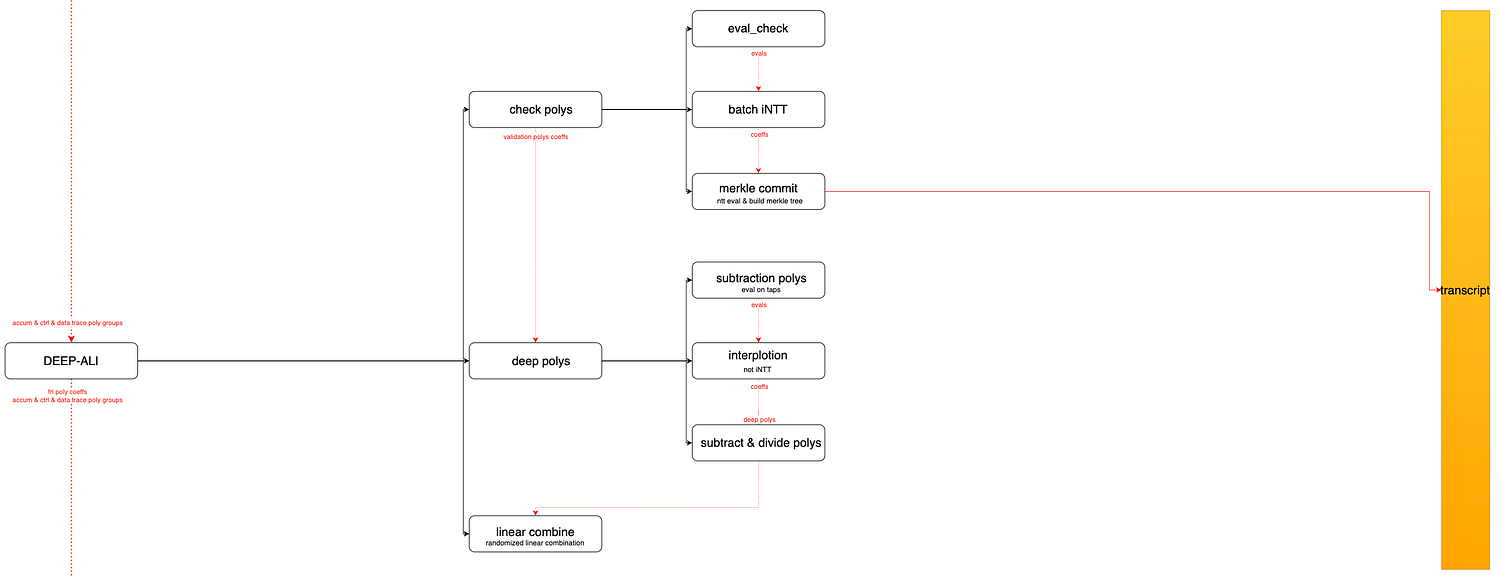
As shown in Figure 5, DEEP-ALI consists of the following steps:
6.1 eval_check, that is, calculating the function value of the check polynomial on the evaluation domain wD0. Because the highest degree of the check polynomial is 4*|H|, the function value needs to be calculated on the evaluation domain wD0 instead of the trace domain H;
6.2 batch iNTT obtains the coefficient of the check polynomial, because the check polynomial is regarded as a polynomial of degree 4*|H| on K, it can be regarded as 16 polynomials of degree |H| on F, thus obtaining a check polynomial polynomial group consisting of 16 polynomials;
6.3 Calculate the function value of each polynomial in the check polynomial group on the commitment domain, and use these function values to construct a merkle tree to obtain the commitment value of the polynomial group;
6.4 Calculate deep polynomials, which is defined as:
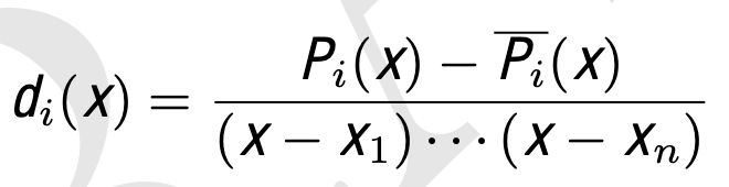
The purpose of deep polys is to ensure that the above check polys are calculated honestly.
We believe that check polys are are calculated honestly if a random value z is taken in the extended domain K, and both sides of the equation in eval_check are equal (there is a soundness error);
If check polys are calculated honestly if and only if the rational function is a polynomial function.
Where Pi is trace poly or check poly;
__Pi is the polynomial obtained by interpolating the function value of Pi at different points required to calculate the “constrained multivariate polynomial function value”, such as xi = ωz, ω is the generator of trace domain H.
6.5 Combine all deep polynomial to get fri polynomials.
7. FRI
The purpose of FRI is to prove that the degree of the fri polynomial is less than or equal to the size of the trace domain H. If deg(fri(X)) ≤ |H|, then the check polynomial is a polynomial whose degree ≤ 4*|H|, and the check polynomial is calculated honestly. Then the elements in the trace satisfy the constrained multivariate polynomial equation system, and the instructions in the segment are executed honestly.
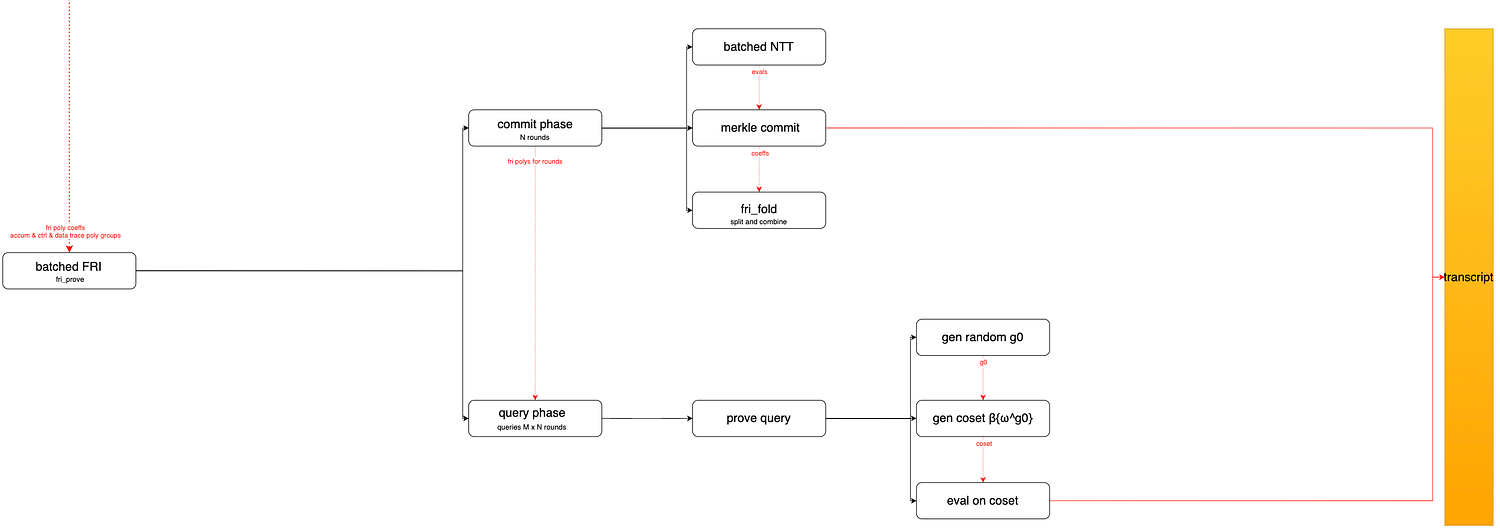
FRI includes commit phase and query phase, as shown in Figure 6, which consists of the following steps:
7.1 commit phase, the degree of fri poly is reduced to 256 in multiples of 16, then there are log(16, deg(fri)) rounds, and the polynomial generated by each round is committed. The following calculations are performed for each round:
7.1.1 fri poly is a polynomial of degree |H| on the extended domain K, which can be regarded as an element of degree |H| on four domains F. The function values of the four polynomials on the commitment domain are calculated through batched NTT;
7.1.2 Using the function value of the fri polynomial on the commitment domain, a merkle tree is constructed to obtain the commitment value;
7.1.3 Split the fri polynomial into 16 parts to obtain 16 sub-polynomials, and then use random linear combine to obtain the fri polynomial of the next round.
7.2 Query phase, for all committed polynomials, including control polynomial, data polynomial, accumulate polynomial, check polynomial, log(16, deg(fri)) round fri polynomial, open proof of these polynomials.
7.2.1 Select a random challenge value g0 in the commitment domain;
7.2.2 Construct the elements in the evaluation set, i.e. g0, g0*16, …, g0^(16*round_n);
7.2.3 Open proof of control polynomial, data polynomial, check polynomial at g0, and open proof of the fri polynomial of round i at g0^(16*round_i).
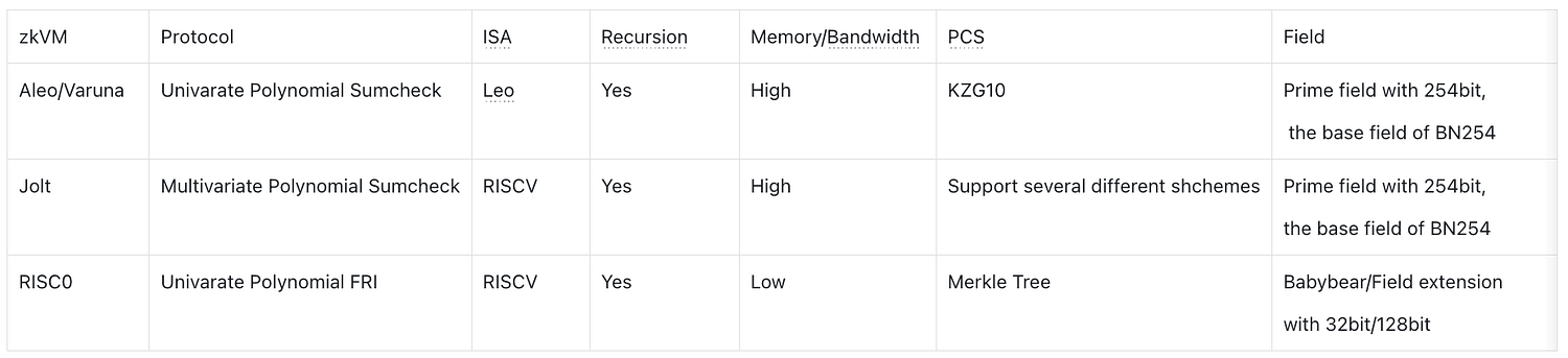
8. Comparison with other zkVMs